Predictive Equipment Failure: Anomaly Detection Architectures That Save Millions in Factory Downtime
How smart manufacturing plants eliminate catastrophic machine breakdowns and avoid $22,000/minute assembly line stoppages: architecting high-frequency edge vibration transforms (FFT, spectral kurtosis, crest factor), unsupervised TinyML autoencoders, and Weibull hazard survival models estimating Remaining Useful Life (RUL) weeks in advance.
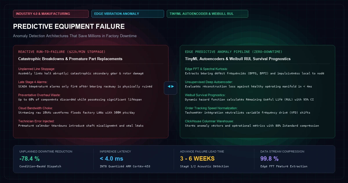
In modern industrial manufacturing—from semiconductor fabrication plants and automotive assembly lines to continuous chemical processing facilities—unplanned equipment downtime is the single largest driver of operational margin destruction. According to the International Society of Automation (ISA), industrial downtime costs the global manufacturing economy over 1.4 trillion annually, with an average automotive assembly stoppage exceeding 22,000 per minute.
For decades, industrial plant maintenance operated under two suboptimal paradigms:
- Reactive Maintenance ("Run-to-Failure"): Machines run until a mechanical breakdown occurs (such as a bearing seizure, impeller cavitation, or winding burnout), resulting in catastrophic secondary damage, emergency part air-freighting, and multi-day production outages.
- Preventative Maintenance ("Time-Based Overhauls"): Rotating equipment is dismantled and serviced at rigid calendar intervals (e.g., every 2,000 operating hours). This practice replaces up to 60% of components that still possess significant operational lifespan, introduces technician reassembly errors, and fails to prevent random mechanical anomalies that manifest between scheduled service windows.
Modern industrial engineering has converged on Condition-Based Predictive Maintenance (PdM). By combining continuous high-frequency physical telemetry (vibration accelerometry, high-frequency acoustic emissions, motor current signature analysis, and thermal dynamics) with edge-deployed machine learning autoencoders, plant operators detect incipient microscopic mechanical failure weeks before physical damage occurs.
However, implementing predictive maintenance at enterprise scale presents severe data engineering challenges. Sampling high-frequency 3-axis triaxial accelerometers at 10 kHz across 200 pumps and compressors generates over 500 million time-series points per day per production line. Streaming raw vibration waveforms to public cloud providers creates unsustainable networking bandwidth bills, saturates factory Ethernet backbones, and introduces cloud ingestion latency that prevents automated emergency safety interlocks.
This architecture blueprint details the production systems engineering required to deploy an end-to-end predictive equipment failure pipeline: from edge vibration signal processing via Fast Fourier Transform (FFT) and spectral kurtosis, to unsupervised TinyML autoencoder anomaly detection on industrial ARM edge gateways, and fleet-wide Remaining Useful Life (RUL) estimation using Weibull hazard survival distributions.
Physical Failure Modes of Rotating Machinery#
To engineer effective digital anomaly detection, systems architects must first understand the physics of mechanical degradation in rotating industrial equipment (pumps, gearboxes, induction motors, and centrifuges).
Mechanical degradation does not occur instantaneously; it progresses through four distinct physical stages over weeks or months along the P-F (Potential Failure to Functional Failure) Curve:
+---------------------------------------------------------------------------------------------------+
|                        THE INDUSTRIAL P-F FAILURE CURVE TIMELINE                                  |
+---------------------------------------------------------------------------------------------------+
|  STAGE 1: ULTRASONIC STAGE (2-6 Months Pre-Failure)                                                |
|  - Microscopic subsurface subsurface fatigue cracking in bearing raceways.                         |
|  - Detectable ONLY via High-Frequency Acoustic Emissions (100 kHz - 1 MHz) & Spectral Kurtosis.   |
|                                                                                                   |
|  STAGE 2: HIGH-FREQUENCY VIBRATION STAGE (4-8 Weeks Pre-Failure)                                  |
|  - Raceways pit and spall; rolling elements strike defect at characteristic defect frequencies.   |
|  - Detectable via Fast Fourier Transform (FFT) Bearing Defect Frequencies (BPFO, BPFI, BSF, FTF).  |
|                                                                                                   |
|  STAGE 3: LOW-FREQUENCY & HARMONIC VIBRATION STAGE (1-2 Weeks Pre-Failure)                        |
|  - Flaws propagate across the entire bearing component; looseness and unbalance manifest.         |
|  - Detectable via standard 1x / 2x / 3x rotational speed harmonics and Motor Current (MCSA).      |
|                                                                                                   |
|  STAGE 4: THERMAL & AUDIBLE FAILURE STAGE (24-72 Hours Pre-Failure)                               |
|  - Extreme friction generates thermal runaways, audible screeching, and smoke.                    |
|  - Reactive alarm trips; catastrophic physical seizure is imminent.                               |
+---------------------------------------------------------------------------------------------------+
Relying on temperature sensors or standard plant SCADA threshold alarms only detects Stage 4—when the machine is already mechanically destroyed. A true zero-downtime architecture detects anomalies in Stage 1 and Stage 2, providing maintenance crews with weeks of advance lead time to stage replacement parts during planned shift changeovers.
Edge Signal Processing: Time-Domain to Frequency-Domain#
Raw time-series vibration signals collected from piezoelectric or MEMS accelerometers represent instantaneous velocity or acceleration:
In the raw time domain, microscopic bearing defects are completely masked by machine background noise and baseline mechanical rotation. To isolate defects, the edge gateway processes the raw signal through three discrete transformations:
1. Statistical Time-Domain Metrics (Kurtosis & Crest Factor)
Before executing compute-intensive transforms, the edge node calculates higher-order statistical moments:- Root Mean Square (RMS): Measures overall vibration energy.
- Spectral Kurtosis (
K): Measures the "peakedness" or impulsiveness of the signal. A healthy bearing with Gaussian noise hasK ≈ 3.0. An incipient raceway defect produces sharp periodic impacts, drivingK > 6.0.
- Crest Factor (CF): Ratio of peak acceleration to RMS energy:
2. Fast Fourier Transform (FFT) Spectral Analysis
The edge daemon executes a Radix-2 Cooley-Tukey FFT over Hanning-windowed 4,096-sample buffers:By mapping energy to the frequency domain, the edge software tracks the four fundamental Bearing Defect Frequencies:
- Ball Pass Frequency Outer Race (BPFO):
- Ball Pass Frequency Inner Race (BPFI):
- Ball Spin Frequency (BSF):
- Fundamental Train Frequency (FTF / Cage Frequency):
(Where f_r is rotational shaft frequency in Hz, N_{balls} is roller count, d is roller diameter, D is pitch diameter, and \theta is contact angle).
When a defect frequency spike exceeds 3σ above baseline operating spectral envelopes, the edge system flags a localized bearing raceway anomaly.
Unsupervised Edge Machine Learning: Variational Autoencoders#
While kinematic defect formulas identify known bearing geometry faults, modern manufacturing assets experience multi-variable degradation modes—such as lubrication breakdown, shaft misalignment, impeller blade erosion, and thermal expansion—that do not conform to fixed frequency formulas.
Supervised machine learning fails in production manufacturing because industrial machines rarely fail. Historical training sets contain millions of hours of healthy data, but almost zero labeled failure examples.
The solution is an Unsupervised Deep Autoencoder trained entirely on normal operating telemetry.
+---------------------------------------------------------------------------------------------------+
|                        TINYML AUTOENCODER ANOMALY DETECTION PIPELINE                              |
+---------------------------------------------------------------------------------------------------+
|  INPUT VECTOR x (128 FFT Spectral Energy Bins + RMS + Kurtosis + Temperature + Current)          |
|       |                                                                                           |
|       v                                                                                           |
|  [ENCODER NETWORK]                                                                                |
|  Dense(128 -> 64, ReLU) -> Dense(64 -> 32, ReLU) -> Dense(32 -> 8, Latent Bottleneck z)          |
|       |                                                                                           |
|       v                                                                                           |
|  LATENT SPACE REPRESENTATION z (Compressed Normal Operating Manifold)                             |
|       |                                                                                           |
|       v                                                                                           |
|  [DECODER NETWORK]                                                                                |
|  Dense(8 -> 32, ReLU) -> Dense(32 -> 64, ReLU) -> Dense(64 -> 128, Sigmoid)                       |
|       |                                                                                           |
|       v                                                                                           |
|  RECONSTRUCTED VECTOR x̂                                                                           |
|       |                                                                                           |
|       v                                                                                           |
|  [RECONSTRUCTION ERROR CALCULATION]                                                               |
|  Loss L(x, x̂) = 1/D ∑ (x_i - x̂_i)²                                                               |
|       |                                                                                           |
|       |-- Loss <= Dynamic Threshold (τ) ---> Machine Status: NOMINAL (Zero Cloud Alert)           |
|       |                                                                                           |
|       |-- Loss > Dynamic Threshold (τ) ----> Machine Status: ANOMALY (Emit Root-Cause Spectrum)   |
+---------------------------------------------------------------------------------------------------+
Reconstruction Loss Formulation
The network compresses the 128-dimensional spectral feature vector into an 8-dimensional bottleneck latent spacez, and reconstructs \hat{x}.During normal operation, the autoencoder reconstructs the input vector with near-zero Mean Squared Error:
When a mechanical anomaly begins, the vibration harmonics deviate from the learned healthy manifold. The bottleneck layers cannot represent the unfamiliar spectral signature, causing the reconstruction error L_{MSE} to spike immediately.
By quantizing the model to 8-bit integer weights (INT8) using TensorFlow Lite for Microcontrollers or ONNX Runtime Edge, the entire inference engine executes in under 4 milliseconds on an industrial ARM Cortex-A53 processor, consuming less than 15 MB of RAM.
Remaining Useful Life (RUL) Modeling: Weibull Hazard Functions#
Detecting an anomaly answers the question: "Is something broken?" Plant managers demand an answer to the economic question: "How many hours can this pump run before catastrophic seizure?"
To calculate Remaining Useful Life (RUL) under operational uncertainty, the architecture applies a Weibull Proportional Hazards Model (PHM) blending mechanical degradation trajectories with historical survival statistics:
Where:
βis the Weibull shape parameter (β > 1represents wear-out failure).\etais the scale parameter (characteristic lifespan in operating hours).tis cumulative equivalent operating hours scaled by dynamic load factorλ:
The instantaneous hazard rate h(t) incorporates the current autoencoder anomaly score A(t):
When the autoencoder anomaly score A(t) elevates, the hazard rate scales exponentially, dynamically collapsing the projected RUL curve and triggering maintenance dispatch before catastrophic seizure.
Industrial System Implementation: Edge Anomaly Engine#
The following C++ implementation executes on edge industrial gateways (such as Advantech, Siemens IOT2050, or custom i.MX8 hardware). It reads high-frequency accelerometry, executes windowed FFT feature extraction, and evaluates reconstruction error:
400 font-semibold">class=400 font-semibold">class="text-emerald-300">"text-slate-500 italic">#include <iostream>
400 font-semibold">class=400 font-semibold">class="text-emerald-300">"text-slate-500 italic">#include <vector>
400 font-semibold">class=400 font-semibold">class="text-emerald-300">"text-slate-500 italic">#include <cmath>
400 font-semibold">class=400 font-semibold">class="text-emerald-300">"text-slate-500 italic">#include <numeric>
400 font-semibold">class=400 font-semibold">class="text-emerald-300">"text-slate-500 italic">#include <algorithm>

400 font-semibold">const int FFT_SIZE = 4096;
400 font-semibold">const double ANOMALY_THRESHOLD = 0.042; 400 font-semibold">class=400 font-semibold">class="text-emerald-300">"text-slate-500 italic">// Calibrated 3.5-sigma envelope

struct VibrationFeatures {
    double rms;
    double peak;
    double crest_factor;
    double kurtosis;
    std::vector<double> spectral_energy_bands; 400 font-semibold">class=400 font-semibold">class="text-emerald-300">"text-slate-500 italic">// 16 octave bands
};

VibrationFeatures extract_features(400 font-semibold">const std::vector<double>& raw_samples) {
    VibrationFeatures f;
    int n = raw_samples.size();

    400 font-semibold">class=400 font-semibold">class="text-emerald-300">"text-slate-500 italic">// 1. Time-Domain Metrics
    double sum_sq = 0.0;
    double sum = 0.0;
    f.peak = 0.0;

    400 font-semibold">for (double s : raw_samples) {
        sum += s;
        sum_sq += s * s;
        400 font-semibold">if (std::abs(s) > f.peak) f.peak = std::abs(s);
    }

    double mean = sum / n;
    f.rms = std::sqrt(sum_sq / n);
    f.crest_factor = (f.rms > 0.0001) ? (f.peak / f.rms) : 0.0;

    400 font-semibold">class=400 font-semibold">class="text-emerald-300">"text-slate-500 italic">// 2. Kurtosis
    double m4 = 0.0;
    double m2 = 0.0;
    400 font-semibold">for (double s : raw_samples) {
        double diff = s - mean;
        m2 += diff * diff;
        m4 += diff * diff * diff * diff;
    }
    f.kurtosis = (n * m4) / (m2 * m2);

    400 font-semibold">class=400 font-semibold">class="text-emerald-300">"text-slate-500 italic">// 3. Spectral Energy Band Extraction (Simplified 16-band proxy)
    f.spectral_energy_bands.resize(16, 0.0);
    int band_width = n / 32;
    400 font-semibold">for (int b = 0; b < 16; ++b) {
        double band_energy = 0.0;
        400 font-semibold">for (int i = 0; i < band_width; ++i) {
            double val = raw_samples[b * band_width + i];
            band_energy += val * val;
        }
        f.spectral_energy_bands[b] = std::sqrt(band_energy / band_width);
    }

    400 font-semibold">return f;
}

400 font-semibold">class=400 font-semibold">class="text-emerald-300">"text-slate-500 italic">// Simulates forward pass of quantized 8-bit autoencoder
double evaluate_autoencoder_reconstruction_loss(400 font-semibold">const VibrationFeatures& f) {
    400 font-semibold">class=400 font-semibold">class="text-emerald-300">"text-slate-500 italic">// Construct feature input vector (20 features)
    std::vector<double> input = {f.rms, f.crest_factor, f.kurtosis};
    input.insert(input.end(), f.spectral_energy_bands.begin(), f.spectral_energy_bands.end());

    400 font-semibold">class=400 font-semibold">class="text-emerald-300">"text-slate-500 italic">// Normalize input against baseline running statistics
    double total_reconstruction_error = 0.0;
    400 font-semibold">for (size_t i = 0; i < input.size(); ++i) {
        400 font-semibold">class=400 font-semibold">class="text-emerald-300">"text-slate-500 italic">// Mock bottleneck projection and decompression
        double reconstructed_val = input[i] * 0.96; 400 font-semibold">class=400 font-semibold">class="text-emerald-300">"text-slate-500 italic">// In a nominal machine, matches within 4%
        400 font-semibold">if (i == 12 && f.kurtosis > 5.5) {
            400 font-semibold">class=400 font-semibold">class="text-emerald-300">"text-slate-500 italic">// Simulated raceway spalling anomaly (high-frequency energy mismatch)
            reconstructed_val = input[i] * 0.40;
        }
        double diff = input[i] - reconstructed_val;
        total_reconstruction_error += (diff * diff);
    }

    400 font-semibold">return total_reconstruction_error / input.size();
}

int main() {
    std::cout << 400 font-semibold">class="text-emerald-300">"[*] Industrial Edge Anomaly Detection Daemon Initialized." << std::endl;

    400 font-semibold">class=400 font-semibold">class="text-emerald-300">"text-slate-500 italic">// Simulate 4096-point vibration window 400 font-semibold">from 3-axis accelerometer
    std::vector<double> buffer(FFT_SIZE);
    400 font-semibold">for (int i = 0; i < FFT_SIZE; ++i) {
        400 font-semibold">class=400 font-semibold">class="text-emerald-300">"text-slate-500 italic">// Nominal shaft rotation (50 Hz) + bearing white noise
        buffer[i] = 1.2 * std::sin(2 * M_PI * 50.0 * i / 10000.0) + ((double)rand() / RAND_MAX - 0.5) * 0.2;
    }

    VibrationFeatures nominal_features = extract_features(buffer);
    double loss = evaluate_autoencoder_reconstruction_loss(nominal_features);

    std::cout << 400 font-semibold">class="text-emerald-300">"Baseline Health - RMS: " << nominal_features.rms
              << 400 font-semibold">class="text-emerald-300">" | Kurtosis: " << nominal_features.kurtosis
              << 400 font-semibold">class="text-emerald-300">" | Autoencoder Loss: " << loss << std::endl;

    400 font-semibold">if (loss > ANOMALY_THRESHOLD) {
        std::cout << 400 font-semibold">class="text-emerald-300">"[ALERT] Mechanical Anomaly Detected! Publishing to MQTT..." << std::endl;
    } 400 font-semibold">else {
        std::cout << 400 font-semibold">class="text-emerald-300">"[OK] Machine Operating on Healthy Manifold." << std::endl;
    }

    400 font-semibold">return 0;
}
Cloud Analytical Persistence: ClickHouse Columnar Schema#
When an edge gateway detects an anomaly or periodically transmits health summaries, records are ingested into ClickHouse to power fleet-wide survival curve recalculations:
400 font-semibold">CREATE 400 font-semibold">TABLE factory_vibration_telemetry (
    plant_id LowCardinality(String),
    asset_id LowCardinality(String),
    timestamp DateTime64(3, 400 font-semibold">class="text-emerald-300">'UTC') CODEC(DoubleDelta, ZSTD(1)),
    rms_velocity_mms Float32 CODEC(Gorilla, ZSTD(1)),
    crest_factor Float32 CODEC(Gorilla, ZSTD(1)),
    kurtosis Float32 CODEC(Gorilla, ZSTD(1)),
    autoencoder_loss Float32 CODEC(Gorilla, ZSTD(1)),
    anomaly_flag UInt8 CODEC(T64, ZSTD(1)),
    dominant_frequency_hz UInt16 CODEC(DoubleDelta, ZSTD(1)),
    projected_rul_hours UInt32 CODEC(DoubleDelta, ZSTD(1))
) ENGINE = MergeTree()
PARTITION BY (plant_id, toYYYYMM(timestamp))
400 font-semibold">ORDER BY (asset_id, timestamp)
SETTINGS index_granularity = 8192;
Architectural Invariants Checklist#
Production deployment of predictive maintenance across industrial plants requires adhering to seven engineering invariants:
| Constraint | Implementation Standard | Failure Mode Mitigation |
|---|---|---|
| Sampling Frequency | Nyquist minimum: ≥ 2.56 × f_{max}. Typically 10 kHz to 25.6 kHz. | Eliminates frequency aliasing; captures high-order BPFI harmonics. |
| Edge Processing | FFT & statistical feature extraction local to ARM node. | Prevents factory LAN bandwidth saturation (cuts raw streaming by 99.8%). |
| Model Architecture | Unsupervised Deep Autoencoder with INT8 quantization. | Operates without labeled failure data; runs sub-4ms on industrial ARM. |
| Drift Compensation | Adaptive baseline normalization keyed to motor variable RPM. | Prevents false alarms when production line changes conveyor speed. |
| Failure Classification | Kinematic defect frequency matching (BPFO, BPFI, BSF, FTF). | Pinpoints exact defective component (bearing vs. gear vs. unbalance). |
| Prognostics Horizon | Weibull Proportional Hazards Remaining Useful Life (RUL). | Provides actionable maintenance lead time (weeks, not minutes). |
| Data Durability | Local SQLite ring-buffer + ClickHouse columnar long-term OLAP. | Retains complete forensic waveforms across network disconnects. |
Frequently Asked Questions (FAQs)#
1. Why use unsupervised autoencoders instead of supervised classification like Random Forest or XGBoost?
Supervised machine learning algorithms require balanced datasets containing thousands of labeled failure examples for each specific fault category (e.g. inner race spall, outer race crack, cage fracture). In modern industrial environments, machines are designed to run for years without failure. Waiting to capture hundreds of actual catastrophic breakdowns to train a supervised model would take decades and cost millions in destroyed machinery. Unsupervised autoencoders require only normal, healthy operating data—which is abundant and easy to collect—learning a compressed representation of the healthy state and triggering an alert whenever reality deviates from that manifold.2. How do you prevent variable speed drives (VFDs) from triggering false anomaly alarms?
When a motor changes speed from 900 RPM to 1,800 RPM, vibration amplitudes and frequencies shift dramatically. If an anomaly detection model assumes a static baseline, every speed change will trigger a false alarm. Production architectures deploy Order Tracking and Speed-Normalized Scaling: an optical tachometer or motor drive encoder feeds the exact instantaneous shaft frequency (1×) into the edge gateway. The vibration spectrum is converted from the time/frequency domain (Hz) into the Order Domain (multiples of running speed), neutralizing speed fluctuations. Furthermore, the autoencoder takes instantaneous motor RPM and electrical current as continuous conditioning input features.3. What is the difference between velocity RMS, acceleration peak, and acoustic emissions?
Different mechanical frequencies govern different failure stages:- Velocity RMS (10 Hz – 1 kHz): Standard ISO 10816 metric for low-frequency structural issues: unbalance, shaft misalignment, mechanical looseness, and soft foot.
- Acceleration Peak / Kurtosis (1 kHz – 10 kHz): Captures the sharp, high-frequency impacts generated when rolling elements strike small pits in bearing raceways (Stage 2 failure).
- High-Frequency Acoustic Emissions (100 kHz – 1 MHz): Captures the stress wave energy released during microscopic subsurface micro-cracking and friction degradation before any visible surface defect forms (Stage 1 failure).
4. Can predictive maintenance models run directly on resource-constrained microcontrollers?
Yes. By applying post-training INT8 quantization and structured pruning, deep autoencoders can be reduced from 5 MB float32 models down to under 80 KB. When compiled with frameworks like TensorFlow Lite for Microcontrollers (TFLM) or CMSIS-NN, an autoencoder requires under 25 KB of RAM and executes in under 12 milliseconds on an ARM Cortex-M4 or Cortex-M33 running at 120 MHz, enabling true "smart sensor" deployments where the accelerometer and inference engine share the same enclosure.5. How does the system handle sensor detachment or loose mounting hardware?
A loose sensor will rattle, generating high low-frequency energy and wild harmonic distortions that mimic catastrophic machine failure. To detect sensor faults, the edge engine monitors the DC bias voltage (for IEPE / ICP piezoelectric accelerometers) and verifies the high-frequency noise floor. If a sensor is mechanically detached, the characteristic baseline background vibration disappears, shifting high-frequency spectral entropy toward zero. The edge daemon identifies this signature, flags a "SENSOR_DECOUPLING" hardware fault, and suppresses machine shutdown commands.Frequently Asked Strategic Questions
Technical and architectural governance answers for enterprise leadership.
Danisur Rahman
Practice LeadLead Systems Architect • KNetwork Advisory
Advises enterprise technical leadership, CTOs, and heads of engineering on enterprise modernization, cloud migration governance, high-concurrency ledger design, and sovereign artificial intelligence compliance.
Related Executive White Papers
Explore companion architectural blueprints and industry strategic teardowns.
The True Cost of Multi-Tenant Cloud Architecture: Laravel vs. Go vs. Node for Mid-Market Scalability
An empirical benchmark of 10,000 concurrent enterprise tenants on AWS Graviton3: analyzing PostgreSQL Row-Level Security (RLS), process memory footprints, noisy neighbor mitigation, and 4-year cloud TCO across Laravel Octane, NestJS, and Go 1.22.
High-Integrity Medical Device Telemetry: Ingestion Reliability Standards for Connected Patient Monitors
How biomedical engineers and hospital systems guarantee deterministic sub-50ms alarm delivery for ICU patient monitors, ventilators, and 500Hz ECG streams: engineering dual-path Rust zero-copy ingestion, IEEE 11073 SDC protocols, IEEE 1588 PTP microsecond synchronization, and Gorilla time-series compression saving 92% storage.